Week 7 – Redlining and Interpolation

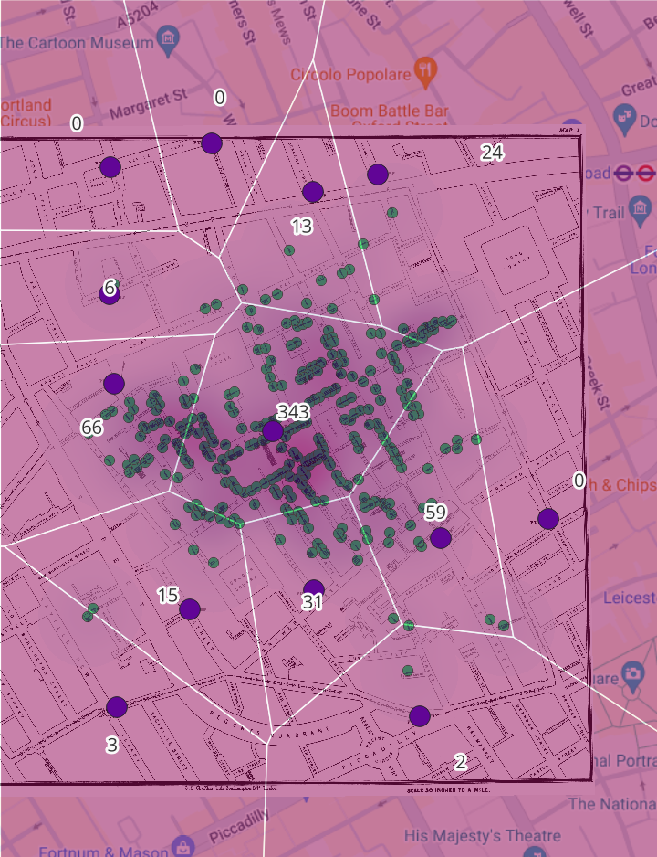
  1. What patterns do you see between mortgage companies and locations that supplied lendeesin Philadelphia?

Here, the total number of mortgages are shown shaded in black. More darkly shaded areas are the ones in which the most mortgages were offered. Berean Savings and Loan Association, a black-owned company, is shown in green. This company’s mortgages were concentrated in areas marked to be high-risk. Metropolitan Life, shown in red, was not a black-owned company. It also sold most of its mortgages in high-risk areas, but the correlation is not quite as dramatic.

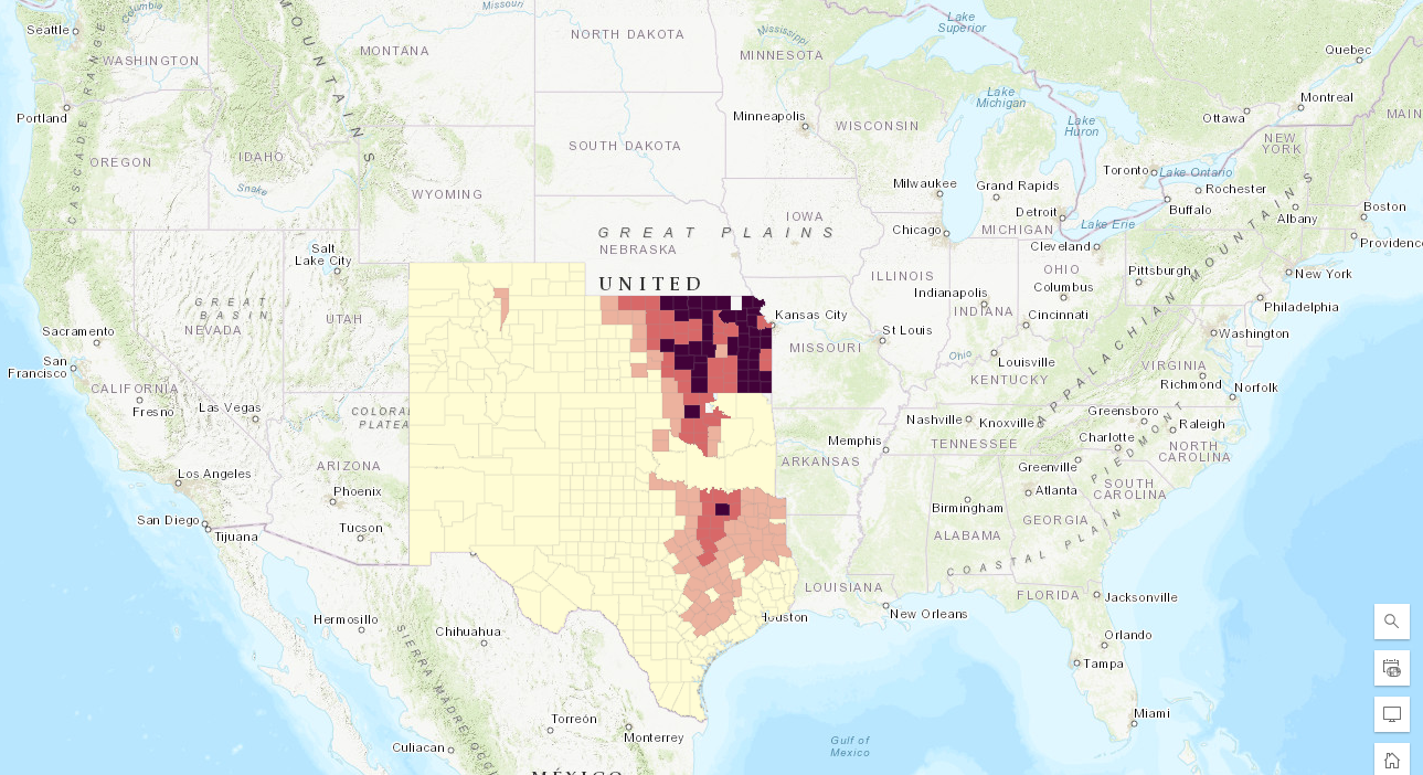
    2. Which regions had the highest interest rates?

    In this map, high interest rates are shown in dark orange. They line up almost exactly with the areas marked as the most high-risk for lenders.

    3. What indication do you see (if any) that HOLC maps caused redlining (as opposed to
    mapping preexisting discrimination)?

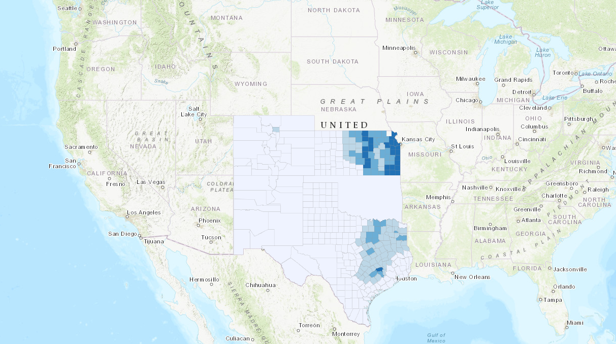
    Here, the percentage of black people living in each neighborhood is represented as a cloropleth map underneath the interest rate layer, with the highest percentages of black residents in purple. Some of the districts the HOLC marked as high risk were in places with few black residents, but the HOCL marked all places with a high percentage of black residents as high-risk. This suggests that while race wasn’t the only factor that caused districts to be marked high-risk, it definitely was a factor.

    4. What additional data layers do you think might supply evidence of discriminatory housing policy/segregated urban development that you don’t have access to in this exercise?

    I’m not very familiar with the intricacies of redlining and honestly, I barely know what a mortgage is, so I don’t think I’m very equipped to identify what data I might be missing. That being said, I think it’d be interesting to be able to see how much money these companies made from collecting interest in different areas. That would help to determine the motivation for their lending patterns and show how much high interest rates affected the likelihood of people taking out loans.

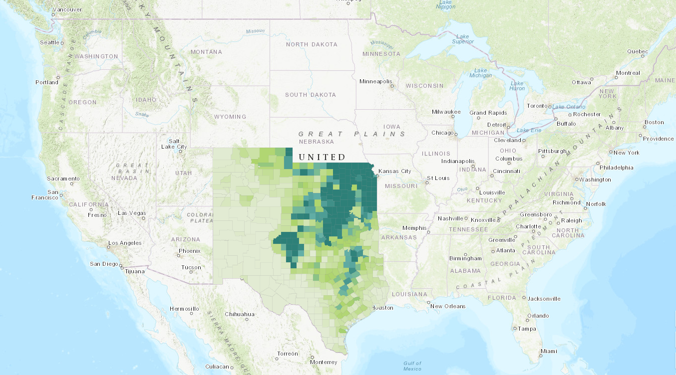
    5. Create one clear, legible map that you think best demonstrates the most compelling
    visualization of redlining in Philadelphia.

    I think that the layer showing interest rates is a very important piece of evidence, but after trying a few different things, I wasn’t able to make it look comprehensible. It looks fine on its own, but when you add any other layer to the same map, it becomes very hard to tell what’s going on.

    My second idea was to show the percentage of black residents in each neighborhood over the HOLC map, but QGIS wasn’t letting me change the opacity of the polygon layers for some reason, so I’ve settled for making the georeferenced HOLC map transparent. It doesn’t look very good, but it does display the same information: neighborhood with a high percentage of black people were always marked as high-risk. The best I could do for readability was get rid of the basemap.

    Week 9 – Intro to ArcGIS Online

    Here are my maps. The higher the percentage of land cultivated, the darker yellow the counties appear.

    1880
    1900
    1940

    The increasing amount of land developed into farmland is definitely visually apparent. Generally, farmland spread to the west, but the areas with the very highest proportion of developed land stay more or less the same. Dark yellow is mostly concentrated in eastern Kansas in all three maps. Although westward expansion and the construction of irrigation infrastructure allowed crops to be grown farther west, the best farmland remained in the northeast.

    Week 6 – Census Data and Cloropleths

    Cotton
    Corn
    Wheat
    Tobacco
    Sugar

    Just glancing at the maps, it’s easy to see that slave labor correlated strongly with the overall amount of crops harvested in each county. This correlation seems to be the strongest when it comes to cotton. The darkest areas on the cloropleth map line up almost perfectly with the cotton output. But while cotton was the biggest contributor, it’s also evident that the other crops were harvested using slave labor; every county with a high slave population outside of the cotton-growing areas correlates with another crop. For example, tobacco affected populations of enslaved people heavily in the northeast and in central Missouri. Sugar farming accounted for high numbers in southern Louisiana.

    If any of these crops weren’t harvested via slavery, it was wheat. Corn, while certainly not correlated as strongly with populations of enslaved people, does seem to have motivated slavery in northern Kentucky. Wheat doesn’t show a clear pattern, but because the patterns for other crops are so strong, I find it hard to believe that wheat just wasn’t harvested with slave labor. Wheat was mostly harvested further north and west, if I remember correctly. It’s likely that the amount of wheat being grown was just so low that it didn’t contribute significantly to the population of enslaved people.

    Practicum 6 – The Dustbowl

    Percentage of Land for Agriculture, by county, 1880
    Percentage of Land for Agriculture, by county, 1900
    Percentage of Land for Agriculture, by county, 1940

    There is a higher concentration of farming in the Northeast in 1880-1900. With an almost insane 72% of land being cultivated in 1900. By the 1940, farming had become more widespread, with most regions that are not desert having at least 10% of their land dedicated to farming. North Texas has also developed substantially since 1900, I wonder if it has something to do with mechanized farming or something else.

    Week 9 Practicum – Evan Murphy

    I think that the most notable change is obviously the inclusion of data on Oklahoma after 1880. I also thought it was notable that overall production in Kansas increased, while it stayed relatively the same everywhere else. Colorado had some increases in the 1940 map but not before.

    Practicum 7 – Mapping Disease

    This heat map demonstrates regions in which there was a heavier concentration of of Cholera deaths. The darker the region the more deaths. Without seeing specific dots indicating death, you can still see a heavy correlation between the broad street pump and amount of deaths.

    This map demonstrates several different factors. Each polygon represents the closest distance to each pump (the purple dot). Each green dot is a death or a number of deaths. Each polygon also lists the amount of death in one region. This map indicates that there is a heavy correlation between the Broad Street Pump and the most deaths in the region.

    I think that Heat Maps would be a good tool to show area impacted. In this case, certain areas were more impacted by the cholera epidemic than others. Areas can also be impacted by severe weather or crime. I think in this case, Voronoi polygons were more useful because it indicated that a pump, which required walking distance, was the source of the disease. Polygons show a better relationship to distance than needed to travel than heat maps.

    I think Voronoi polygons could specifically be useful in my project because I am mapping access to schools. Distance to schools, and distance to a “good” school has a lot of determination on outcomes like future earnings. Mapping the access to good schools could help demonstrate a pattern in student outcomes in different neighborhoods of Omaha.

    Week 9 Practicum – The Dust Bowl

    The Dust Bowl was an event that impacted Central and Southern States during the 1930s. It has been attributed to a number of different causes, including the over cultivation of land during droughts.

    This is a map of the total cultivation of land in 1880 in the states most impacted by the Dust Bowl. Land Cultivation is primarily centered around eastern Kansas and eastern Texas.

    This is a map of the total cultivation of land in 1900 in the states most impacted by the Dust Bowl. Land Cultivation has expanded to include regions of central Kansas and central Oklahoma, while the area of Texas has widely remained the same, but the amount of cultivation in each individual county has changed

    This is a map of total cultivation of land in 1940 in the states most impacted by the Dust Bowl. Cultivation has further expanded to include most of Kansas, Oklahoma, and eastern and central Texas. It has also more heavily expanded into Colorado and New Mexico.

    I think this map helps to prove the theory that land cultivation accompanied by droughts helped contribute to the dustbowl. There is a definite increase in land cultivation across this area, and over cultivation accompanied by abnormal weather conditions can be a recipe for disaster in agricultural areas.

    Mapping Ecological and Economical Disaster

    1880

    1900

    1940

    The most obvious change to me was Oklahoma, as we can see in the 60 years of these maps, more data was being collected. This can be verified because the data had become more split up to provide more accuracy. since 1880 it is known that the population in Midwestern states has grown significantly and as the population expanded so did the land use. These maps show an understandable display oof the cultivation od land use through 60 years.

    css.php